1.9 Summarizing Effect Estimates in Inferential Analyses

When users wish to perform an inferential analysis, they must first run the QRP at a data site (also referred to herein as data partner, DP) and return risk-set-level datasets²³. As part of the QRP, the user has already chosen the study design—e.g., exposures with follow-up time or medical product use during pregnancy—and balancing technique—e.g., propensity score [PS] matching or weighting, or covariate stratification. The QRP Reporting Tool then: 1) aggregates the datasets, 2) subsets the data into any requested subgroups, 3) selects one or more confounding adjustment options, 4) runs regressions to generate effect estimates, and 5) calculates additional measures of frequency and association. The specific methods used are based upon the study design and balancing technique requested in the QRP, as well as the level of data returned.

The QRP Reporting Tool additionally computes and outputs aggregated patient characteristics, propensity score distributions, Kaplan-Meier curves, high-dimensional propensity score (hdPS) variable selection information, and the distribution of patient weights where applicable. Each of these features is discussed in other sections. This section will focus on the computation and summary output of effect estimates and risk metrics.

For the purposes of this section, we refer to patients in the exposed group as “treated,” patients in the comparator group as “untreated,” and the health outcome(s) of interest under study as “event(s)” although we acknowledge that in some studies the comparator group may not actually be untreated and the health outcome(s) of interest may not be events.

1.9.1 Output

1.9.1.1 Aggregated Datasets

After subsetting data according to any requested subgroups, the QRP Reporting Tool aggregates the individual- or risk-set-level datasets that were output from the QRP and will be used to perform confounding adjustment and calculate effect estimates and risk metrics. These datasets, and the circumstances under which they are aggregated by the QRP Reporting Tool are described in Table 1.12. Of note, only risk sets for cohorts whose PS model converged are included in aggregated datasets (see “User Options” for more information). All datasets are stored in the “msocdata” folder within the QRP Reporting Tool file structure. For more information on the formatting and output of aggregated datasets, see the “Output Datasets” section in this documentation.

Table 1.12: QRP Datasets Aggregated in Inferential Analysis Reporting
Dataset	Description	Aggregated
runid_riskdiffdata	De-identified, aggregated data that will be used to calculate unadjusted and adjusted risk differences for the overall sample, the matched sample, the overall sample stratified by percentile, pre-specified subgroup, and the matched sample not stratified on MATCHID (when requested). Also used to calculate odds ratios in studies of medical product use during pregnancy.	Always
runid_risksetdata	Risk sets for the entire sample, the matched sample, the entire sample stratified by percentile, pre-specified subgroup, and the matched sample not stratified on MATCHID (when requested).	Only when performing a study of exposures with follow-up time, not for studies of medical product use during pregnancy.
runid_adjusted	Individual-level unadjusted and adjusted samples.	Only when individual-level data is returned from the QRP.
runid_marginalweights	Weighted sums for the risk sets to compute adjusted hazard ratios (HRs) and robust 95% confidence intervals overall and by pre-specified subgroup. There is one row per risk set.	Only when QRP constructed a PS stratum weighted or inverse probability weighted (IPW) cohort.
runid_weightdistribution	Distribution of stratum/IP weights, after truncation and/or trimming (if user-requested) overall and by pre-specified subgroup.	Only when QRP constructed a PS stratum weighted or IPW cohort
runid_varinfo	All covariates considered for variable selection in hdPS,a description of the variables, an indicator for its source data dimension, statistics used to determine variable selection, an indicator for whether or not the variable was selected into the hdPS model. Output overall and by pre-specified subgroup.	Only when QRP constructed a cohort based on hdPS.

1.9.1.2 Confounding Adjustment

Before computing effect estimates of the treatment(s) on the event(s) of interest, users have several options within the QRP Reporting Tool to adjust for confounding: site-only, conditional matched, unconditional matched, unconditional stratified, and inverse probability weighted. The method of adjustment is based on the type of risk set created in the QRP (and also the user’s request, as noted in the “User Options” section below).

When all eligible treated and untreated patients are included in the model without any additional adjustment for confounders, we refer to the analysis as “site-adjusted” only. In matched or stratified analyses, the QRP Reporting Tool may restrict the analytical population to only those patients who were matched or stratified and rely on the risk sets (or individual-level datasets) that were created within QRP to create either conditional or unconditional effect estimates as appropriate to the study design and balancing technique (see Table 1.13).

To review, the QRP creates site-specific risk-set-level datasets for non-weighted cohorts in studies of exposures with follow-up time and uses risk difference datasets for studies of medical product use during pregnancy. In addition to creating site-specific risk sets or risk difference datasets (which include all eligible treated and untreated patients), the QRP also creates “conditional” datasets, which are restricted to patients who were either matched or assigned a stratum and which calculates probabilities and counts conditioned on the matched set or stratum (except in fixed-ratio PS-matched studies of medical product use during pregnancy). When requested in qrp.PSMatchingFile, the QRP also creates risk-set-level datasets restricted to matched or stratified patients, but with probabilities and counts not conditioned on matched set or stratum. These are known as “unconditional” risk sets, and can only be requested in the QRP for fixed-ratio PS-matched cohorts in studies of exposures with follow-up time due to the imbalance in covariate distribution between treated and untreated cohorts that result from variable-ratio PS matching. Because the QRP Reporting Tool currently only calculates site-adjusted effect estimates for variable-ratio PS-matched studies of medical product use during pregnancy, it is not recommended to conduct the aforementioned analysis.

When the matched or stratified population is used in the QRP Reporting Tool analysis using risk set data created in the QRP by conditioning on the set or stratum, the QRP Reporting Tool indicates that the analysis is “conditional,” and “unconditional” otherwise. Unconditional results are output by default for PS-matched studies of medical product use during pregnancy and can be requested using the L2ComparisonFile for fixed-ratio PS-matched studies of exposures and follow-up time. Because all patients in a matched set are censored when the set becomes uninformative (see QRP documentation for more information on how risk sets are created), the total person-time in a PS-matched cohort conditioned on the matched set—i.e., a conditional analysis—will be less than the total person-time in an unconditional analysis of a PS-matched cohort.

To adjust for confounding with weighted cohorts in studies of exposures with follow-up time—i.e., PS-stratum and inverse probability weighting [IPW] techniques—the QRP Reporting Tool runs a weighted regression model stratified by data partner, where weights are a function of the PS model specified in the QRP.

1.9.1.3 Effect Estimation

For studies of exposures with follow-up time, the QRP Reporting Tool performs a time-to-event analysis and computes hazard ratios (HRs) and associated 95% confidence intervals (CIs) for PS-matched, PS-stratified, covariate-stratified, PS stratum-weighted, and inverse probability of -weighted (IPW) cohorts using either Cox proportional hazards (for individual-level data) or the equivalent case-centered logistic regressions (for risk-set-level data). Because studies of medical product use during pregnancy in Sentinel do not currently handle time-to-event outcomes, the QRP Reporting Tool uses either traditional logistic regressions or the Cochran-Mantel-Haenszel method to estimate odds ratios (ORs) and 95% CIs. Risk metrics are calculated using the same method regardless of study design. A prototypical effect estimate table is shown in Figure 1.4.

In cohorts that were balanced using weights, the QRP Reporting Tool only estimates HRs for the weighted population but does output measure of frequency and association for both the unweighted and weighted groups. Because users can specify the effect estimate targeted by the weighting technique (see the QRP documentation for more information), all tables output from the QRP Reporting Tool that contain results from weighted cohorts include a footnote that defines the meaning of the weighting scheme.

When users request demographic subgroups or subgroups based on levels of covariates previously specified in qrp.CovariateCodesFile, the QRP Reporting Tool additionally computes effect estimates stratified by subgroup. Measures of frequency and association in subgroup analyses are output for all cohorts (non-weighted and weighted).

Table 1.13: Effect Estimate Confounding Adjustment
Study design	Balancing technique	Population	Confounder adjustment	Statistical analysis	Effect estimate output	Risk metric output
Exposures with follow-up time	FR PS matching*	All treated and untreated	Site-adjusted	Cox proportional hazards or case-centered logistic regression**	HRs, 95% CI	Y
		All matched	Conditional	Cox proportional hazards or case-centered logistic regression**	HRs, 95% CI	Y
		All matched	Unconditional	Cox proportional hazards or case-centered logistic regression**	HRs, 95% CI	Y
	VR PS matching, unweighted PS stratification, CS	All treated and untreated	Site-adjusted	Cox proportional hazards or case-centered logistic regression**	HRs, 95% CI	Y
	VR PS matching, unweighted PS stratification, CS	All matched or stratified	Conditional	Cox proportional hazards or case-centered logistic regression**	HRs, 95% CI	Y
	PS stratum weighting, IPW	Unweighted	N/A	N/A	N/A	Y
	PS stratum weighting, IPW	Weighted	N/A	Hybrid quasi-Newton least squares	HRs, robust 95% CI	Y
Medical product use during pregnancy	FR PS matching***	All treated and untreated	Site-adjusted	Traditional logistic regression	ORs, 95% CI	Y
	FR PS matching***	All matched	Unconditional	Traditional logistic regression	ORs, 95% CI	Y
	Unweighted PS stratification, CS**	All treated and untreated	Site-adjusted	Traditional logistic regression	ORs, 95% CI	Y
	Unweighted PS stratification, CS**	All matched or stratified	Conditional	Cochran-Mantel-Haenszel	Conditional	Y

CS: covariate stratification; FR: fixed-ratio; IPW: inverse probability weighting; PS: propensity score; VR: variable ratio
* Users can choose whether to output the conditional and/or unconditional analysis by setting the appropriate parameters in L2 Comparison File, assuming the requested analysis was also specified in qrp.PSMatchingFile.
** The QRP Reporting Tool uses Cox proportional hazards regression when individual-level data was returned from the QRP, and case-centered logistic regression otherwise
*** Because only site-adjusted results are output for VR PS matching in studies of medical product use during pregnancy, this balancing technique is not shown here

1.9.1.4 Risk Metrics

In addition to effect estimates generated from regressions, the QRP Reporting Tool also outputs various risk metrics and summary information for inferential studies, as shown in Figure 1.4 below. Of note, because studies of medical product use during pregnancy in Sentinel do not currently handle time-to-event outcomes, the following metrics are not displayed for these studies: person-years at risk (total and average), person-days at risk, as well as incidence rate (and incidence rate difference) per 1,000 person-years.

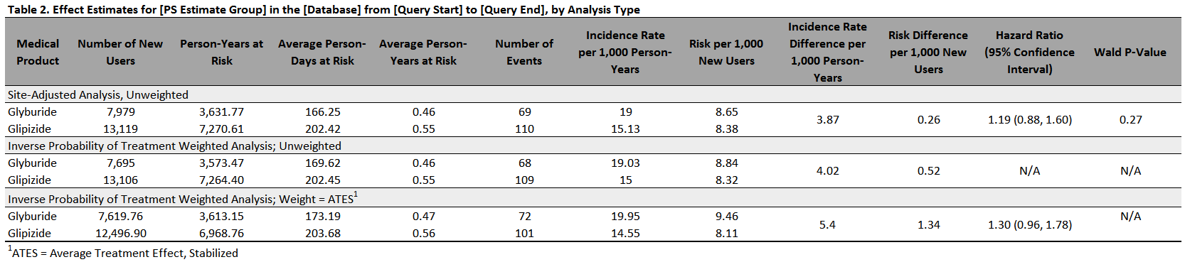
Figure 1.4: Sample Effect Estimates Table

1.9.2 User Options

As with most features in the QRP Reporting Tool, users can specify which data to include, and whether to stratify the output by data partner using the QRP Report Create Report File. Additional user options pertaining to effect estimates and risk metrics are described below.

1.9.2.1 Aggregating Datasets

Users should include all analysis groups for which they would like effect estimates output in the QRP Report L2 Comparison File. Any groups not specified therein will not have effect estimates calculated.

For each PS model run in the QRP, various statistics are output in the dataset qrp.RUNID_estimates. Because only cohorts created from models that converged are aggregated and used to compute effect estimates in the QRP Reporting Tool, users must specify what convergence statuses they would like to use to define “convergence” for the purposes of their study. Using the QRP Report L2 Comparison File, users may choose any combination of the following: convergence satisfied, missing initial values for some parameters, quasi-complete separation, complete separation, ridging has failed to improve the likelihood, iteration limit reached without convergence, missing initial values for some of the parameters, line search has failed to improve the likelihood, improper initial values for the intercept estimates, improper initial values for estimating the model parameters.

1.9.2.2 Confounding Adjustment

While the majority of analytical choices are made before the QRP is executed, users requesting analyses for fixed-ratio PS-matched cohorts in studies of exposures with follow-up time must re-iterate their request for conditional or unconditional confounding adjustment analyses using the QRP Report L2 Comparison File.

When individual-level data is returned, users may additionally specify that other confounders not included in the PS model (including demographic characteristics) be included in the event regression model using the QRP Report L2 Comparison File, providing that these confounders were also specified before the execution of QRP in qrp.CovariateCodesFile.

1.9.2.3 Adjustment for Potential Selection Bias in Studies of Medical Product Use During Pregnancy

Because the QRP includes only live births in studies of medical product use during pregnancy, it by necessity excludes stillbirths and incomplete pregnancies. This may bias the regression results toward the null resulting in an underestimation of the true association between a treatment and event of interest.

Thus, when a study of medical product use during pregnancy was performed in the QRP, the user may request that the QRP Reporting Tool adjusts for potential selection bias in an analysis of treated and untreated pregnancy cohorts. To do so, for each analysis group and effect estimation technique, they must specify the probability for case and non-case selection (see Table 1.14) among the treated and untreated using the QRP Report Selection Probabilities File. The QRP Reporting Tool will use these inputs later to adjust computed odds ratios and 95% confidence intervals.

Table 1.14: User-Specified Selection Probabilities
User-Specified Probability	Description
S₁₁	Probability of case selection among the treated
S₀₁	Probability of case selection among the untreated
S₁₀	Probability of non-case selection among the treated
S₀₀	Probability of non-case selection among the untreated

1.9.2.4 Redaction

Users may choose to redact certain columns from the effect estimate tables (an example of which is shown in Figure 1.4) by specifying their choices in the QRP Report Create Report File. Users may choose from the following redaction options:

Redact all information on the event of interest by redacting the number of events in the treated and untreated groups and all risk metrics
Redact most of the information on the event of interest by summing the events over treated and untreated groups and redacting all risk metrics
Redact all information on person-time by redacting total and average person-time as well as all effect estimates
Redact any combination of the above

1.9.3 Calculations

This section provides in-depth explanations of the calculations used by the QRP Reporting Tool to provide effect estimates and risk metrics. In all equations, assume the following:

There are $n$ patients included in the aggregated dataset from $K\ (k=1,\ldots,k)$ data sites such that $n_k\ (i=1,\ldots,n)$ patients are contributed from each data site.
$A$ is the binary treatment indicator ($A=1$ if treated and $A=0 $if untreated) such that $n_A$ is the number of patients in each treatment group
$T=min\left(T^\ast,C\right)$ is the actual observed time where $T^\ast$ is the time at which a patient experiences an event, and $C$ denotes a patient’s observation terminating due to anything other than the event of interest.
$Y$ is the binary event indicator which takes the value 1 if ${T=T}^\ast$—i.e., the patient experiences the event—and 0 if $T=C$—i.e., the patient is censored. $n_{Y=1}$ is the number of patients who experience the event of interest.
$\mathbb{X}$ is the vector of covariates, $x (m=1,\ldots,m)$ included in a given model and $\mathbb{B}$ is the vector of regression parameters associated with the explanatory variables, composed of $\beta\ (m=1,\ldots,m)$.

1.9.3.1 Cox Proportional Hazards Regression

As noted above, when individual-level data is returned from the QRP in non-weighted studies of exposures with follow-up time, the QRP Reporting Tool runs a Cox proportional hazards regression on the qrp.RUNID_adjusted dataset from QRP to compute HRs and 95% confidence intervals. It fits the Cox model by maximizing the partial likelihood and computes baseline survivor functions using the Breslow estimate. In the case of tied failure times, the Breslow approximation of the exact method is used.

Definition 1.2 (Cox Propotional Hazards Regression) Each data partner is assumed to have its own baseline hazard function, and models are stratified by data partner to adjust for inter-site differences. Under these stratified models, the hazard function for the $i^{th}$ patient from the $k^{th}$ data site is expressed as in Equation (1.12) where $\lambda_{k0}\left(t\right)$ is the arbitrary and unspecified baseline hazard function for the $k^{th}$ data partner, $\mathbb{X}_{ik}$ is the vector of explanatory variables for the patient, and $\mathbb{B}$ is the vector of regression parameters associated with the explanatory variables. $\mathbb{B}$ is assumed to be the same for all patients.

Equation (1.12): Hazard Function

\[\begin{equation} \lambda_{ik}\left(t\right)=\lambda_{0k}\left(t\right)e^{\mathbb{X}_{ij}^\prime\mathbb{B}} \tag{1.12} \end{equation}\]

Equation (1.13): Log-Hazard Function

\[\begin{equation} \ln{\left[\lambda(t|A,x)\right]}=\ln{\left[\lambda_0(t)\right]+\beta_AA+\beta_1x_1+\ldots+\beta_mx_m} \tag{1.13} \end{equation}\]

Given the log-hazard function in Equation (1.13), the hazard ratio $\theta$ is defined as the ratio of the hazard for the treated patients to the hazard for the untreated patients. To obtain the log-hazard ratio $(\ln{\left[\theta\right]})$, the QRP Reporting tool uses the SAS PROC PHREG procedure to estimate $\beta_A$ using the partial likelihood function, eliminating the need to know the baseline hazard while at the same time accounting for right censoring as shown in Figure (1.14).

Equation (1.14): Log-Hazard Ratio

\[\begin{equation} \ln{\left[\theta\right]}\equiv\ln{\left[\theta\left(A=1,A=0\right)\right]}=\ln{\left[\lambda\left(t\middle| A=1\right)\right]}-\ln{\left[\lambda\left(t\middle| A=0\right)\right]}=\beta_A \tag{1.14} \end{equation}\]

1.9.3.2 Case-Centered Logistic Regression

When risk set-level data is returned from a non-weighted study of exposures with follow-up time, the QRP Reporting Tool fits case-centered logistic regressions to the aggregated QRP datasets to evaluate the association between treatments and events of interest. These types of regressions have been shown to return effect estimates and error equal to what would have been estimated with a Cox proportional hazards regression on patient-level data.[3]

Briefly, the model is known as “case-centered” because it focuses on the “cases,” or the patients who experienced the event of interest. The observed odds of treatment are compared with the expected odds of treatment to examine whether a higher-than-expected proportion of cases receive treatment.

To perform this technique, the QRP Reporting Tool uses an aggregated dataset of each Data Partner’s output in qrp.RUNID_risksetdata, which includes only cases with one record for each case. In addition to identifying the treatment status of each case, this aggregated dataset also includes the expected probability of treatment for each case, which was calculated during the QRP execution by computing the probability of treatment for all non-cases who were at-risk and under follow-up at the time of the case—i.e., in the same risk set—(see QRP functional documentation for more information).

Definition 1.3 (Case Centered Logistic Regression) To calculate HRs and associated 95% CIs in this technique, the QRP Reporting Tool first uses the probability of treatment among non-cases, $P(A=1|Y=0)$, as the expected probability of treatment among cases, and then transforms that into the expected log-odds of treatment among cases $(logit{P_0})$ as shown in Equation (1.15). . This term is used as the offset in an intercept-only logistic regression where the dependent variable is observed odds of treatment among cases, $logit{P_1}$, as shown in Equation (1.16) and Equation (1.17). Therefore, the exponentiation of the intercept term, $\beta_0$, provides a hazard ratio for the association between treatment and the event of interest.

Equation (1.15): Log-odds of Expected Treatment Probability Among Cases

\[\begin{equation} logit{P_0}=logit{\left[P(A=1|Y=0)\right]}=\ln{\left[\frac{P(A=1|Y=0)}{1-P(A=1|Y=0)}\right]} \tag{1.15} \end{equation}\]

Equation (1.16): Log-odds of Observed Treatment Probability Among Cases

\[\begin{equation} logit{\left(P_1\right)}=logit{\left(\pi_{K\left(1\right)|Y(1)}\right)}=\ln{\frac{\pi_{K\left(1\right)|Y(1)}}{1-\pi_{K\left(1\right)|Y(1)}}} \tag{1.16} \end{equation}\]

Equation (1.17): Case-Centered Logistic Regression Model

\[\begin{equation} logit{\left(P_1\right)}=logit{\left(P_0\right)}+\beta_0 \tag{1.17} \end{equation}\]

The logistic regression model is constructed using the SAS procedure PROC GENMOD assuming a binomial distribution and logit link. Of note, the logistic regression model drops all cases for whom the expected probability of treatment is 0 or 1; these are noninformative cases and do not contribute to the analysis.

1.9.3.3 Hybrid Quasi-Newton Least Squares

For studies of exposures with follow-up time that utilize weighting as balancing technique—i.e., IPT- or PS stratum weighted), the QRP Reporting Tool still uses a Cox proportional hazards regression model but applies a different method.

Definition 1.4 (Hybrid Quasi-Newton Least Squares) Based on the propensity score, $e=P\left(A=1|\mathbb{X}\right)$, the inverse probability weight is defined within the QRP as the inverse of the probability of receiving the observed treatment—i.e., $w=w_{ipw}=\frac{A}{e}+\frac{1-A}{1-e}$ where the propensity score is estimated by fitting a logistic regression model relating $A$ to $\mathbb{X}$. The use of $w_{ipw}$ within the QRP results in a “pseudo-population” in which the treatment variable is unrelated to the measured baseline characteristics. The QRP Reporting Tool can then use a Cox regression model weighted by $w_{ipw}$ to yield a marginal hazard ratio estimate and robust sandwich variance that accounts for the confounding effects of baseline covariates.[4]

As a result, the stratified Breslow-type weighted partial likelihood score function equals the summation of $K$ site-specific functions, yielding the score equation for the common log hazard ratio, $\theta$, seen in Equation (1.18) where $\mathcal{R}_j\left(k\right)$ is the risk set for the $j^{th}$ distinct observed event time, $d\left(k\right)$, in site $k$.

Equation (1.18): Score Equation for Log Hazard Ratio

\[\begin{equation} \sum_{k=1}^{K}\sum_{j=1}^{d(k)}{\left\{\sum_{i:i\epsilon D_j(k)}{{\hat{w}}_iA_i}-\sum_{i:i\epsilon D_j(k)}{{\hat{w}}_i\frac{\sum_{l:l\epsilon\mathcal{R}_j(k)}{{\hat{w}}_l{A_le}^{A_l\theta}}}{\sum_{l:l\epsilon\mathcal{R}_j(k)}{{\hat{w}}_le^{A_l\theta}}}}\right\}=0} \tag{1.18} \end{equation}\]

To obtain the log hazard ratio estimate, $\hat{\theta}$, the QRP Reporting Tool solves Equation (1.18) for $\theta$ using the Hybrid Quasi-Newton method of nonlinear least squares in the NLPHQN package in SAS PROC IML. Note that after manipulation, Equation (1.18) is equivalent to Equation (1.19) for each distinct observed event time, $d\left(k\right)$, at each site $k$.

Equation (1.19): Score Equation for Log Hazard Ratio for Each Distinct Event Time at Each Site

\[\begin{equation} \left\{\sum_{i:i\epsilon D_j\left(k\right),A_i=1}{\hat{w}}_i\right\}-\left\{\left[\sum_{i:i\epsilon D_j\left(k\right)}{\hat{w}}_i\right]\left[\frac{e^\theta\sum_{l:l\epsilon\mathcal{R}_j\left(k\right),A_l=1}{\hat{w}}_l}{\left(e^\theta\sum_{l:l\epsilon\mathcal{R}_j\left(k\right),A_l=1}{\hat{w}}_l\right)+\left(\sum_{l:l\epsilon\mathcal{R}_j\left(k\right),A_l=0}{\hat{w}}_l\right)}\right]\right\}=0 \tag{1.19} \end{equation}\]

Thus, to estimate $\hat{\theta}$ the Reporting Tool only needs information on the total weights of treated events $(\sum_{i:i\epsilon D_j\left(k\right),A_i=1}{\hat{w}}_i)$, total weights of events $(\sum_{i:i\epsilon D_j\left(k\right)}{\hat{w}}_i)$, total weights of treated patients $(\sum_{l:l\epsilon\mathcal{R}_j\left(k\right),A_l=1}{\hat{w}}_l)$, and total weights of untreated patients $(\sum_{l:l\epsilon\mathcal{R}_j\left(k\right),A_l=0}{\hat{w}}_l)$ for each observed event time at each data partner.All of this information is returned in qrp.RUNID_marginalweights after each data partner’s QRP execution.

1.9.3.4 Traditional Logistic Regression Adjusted for Potential Selection Bias in Studies of Medical Product Use in Pregnancy

When individual or risk-set level data is returned from non-stratified studies of medical product use in pregnancy, the QRP Reporting Tool uses logistic regressions to estimate the effect of treatment on the event of interest. Because no measure of time is included in studies of medical product use in pregnancy and the outcome is binary, the QRP Reporting Tool estimates ORs and corresponding 95% CIs.

The QRP Reporting tool uses aggregated data from qrp.RUNID_adjusted to conduct regressions when patient-level data is returned from the QRP and qrp.RUNID_riskdiffdata otherwise. The logistic regression model is constructed using the SAS procedure PROC GENMOD assuming a binomial distribution and logit link. Of note, if risk set-level data was returned from the QRP, the QRP Reporting Tool will first transform the aggregated dataset in order to identify treated and untreated groups.

Definition 1.5 (Traditional Logistic Regression Adjusted for Potential Selection Bias in Studies of Medical Product Use in Pregnancy) If $p=P(Y=1) $ at each of $K (k=1,\ldots k)$ data sites, then we can fit the logistic regression model shown in Equation (1.20) where the dependent variable is the expected odds of the event and independent variables include: 1) all specified covariates $x_1$through $x_m$, 2) the data site $K_k$, and 3) the treatment status $A_i$. The exponentiation of the parameter $\beta_A$ will provide an odds ratio for the association between treatment and the event of interest adjusted for the data site and all specified covariates.

Equation (1.20): Traditional Logistic Regression

\[\begin{equation} logit{p}=\ln{\frac{p}{1-p}=}\beta_0+\beta_AA_i+\beta_KK_k+\beta_1x_1+\beta_2x_2\ldots+\beta_mx_m \tag{1.20} \end{equation}\]

The QRP Reporting Tool adjusts for the selection bias likely introduced in studies of medical product use during pregnancy as described in previous work[5] and developed elsewhere.[6,7] Briefly, after calculating the odds ratio using either a traditional logistic regression or the Cochran-Mantel-Haenszel estimate, the QRP Reporting Tool employs user-specified values from the QRP Report Selection Probabilities File as shown in Table 1.14 to estimated adjusted odds ratios (AOR; see Equation (1.21)) and confidence intervals ($95%CIadj$ where SE is the standard error; see Equation (1.22)).

Equation (1.21): Odds Ration Adjusted for Selection Bias

\[\begin{equation} AOR=OR\left(\frac{S_{10}S_{01}}{S_{11}S_{00}}\right) \tag{1.21} \end{equation}\]

Equation (1.22): Confidence Intervals Adjusted for Selection Bias

\[\begin{equation} 95\%CI_{Adj}=AOR1.96\pm\left(SE_{OR}\right) \tag{1.22} \end{equation}\]

1.9.3.5 Cochrane-Mantel-Haenszel

For studies of medical product use during pregnancy, if there are fewer than four events in the population or the QRP used a stratum balancing technique, the QRP Reporting Tool employs the Cochran-Mantel-Haenszel method to calculate a common odds ratio and 95% confidence interval across strata. This is employed through the use of the CMH option in the SAS PROC FREQ procedure.

1.9.3.6 Risk Metrics

Risk metrics are computed for all inferential study designs regardless of balancing technique used in the QRP (see Table 1.13 above). In each case, the QRP Reporting Tool sums the number of treated and untreated patients, number of events among treated and untreated patients, and follow-up time among treated and untreated patients using data aggregated by analysis group in each data partner’s qrp.RUNID_riskdiffdata output dataset. Each risk metric is calculated as shown in Table 1.15.

Table 1.15: Risk Metric Calculations
Risk Metric	Calculation
Number of patients in a treatment group	$n$
Total follow-up time, person-years	$\frac{T^\ast}{365.25}$
Average follow-up time, person-years	$\frac{\left(\frac{T^\ast}{n}\right)}{365.25}$
Number of events	$n_{Y=1}$
Incidence rate per 1,000 person-years	$\frac{\left(\frac{n_{Y=1}}{T^\ast}\right)}{365.25}\times1000$
Incidence rate difference per 1,000 person-years	$\frac{\left[\left(\frac{n_{Y=1\|A=1}}{T_{A=1}^\ast}\right)-\left(\frac{n_{Y=1\|A=0}}{T_{A=0}^\ast}\right)\right]}{365.25}\times1000$
Risk	$\left(\frac{n_{Y=1}}{n}\right)\times1000$
Risk difference	$\left[\left(\frac{n_{Y=1\|A=1}}{n_{A=1}}\right)-\left(\frac{n_{Y=1\|A=0}}{n_{A=0}}\right)\right]\times1000$

References

Fireman B, Lee J, Lewis N, et al. Influenza Vaccination and Mortality: Differentiating Vaccine Effects From Bias. American Journal of Epidemiology 2009;170:650–6. doi:10.1093/aje/kwp173

Shu D, Yoshida K, Fireman BH, et al. Inverse probability weighted Cox model in multi-site studies without sharing individual-level data. Statistical Methods in Medical Research 2020;29:1668–81. doi:10.1177/0962280219869742

Huybrechts KF, Palmsten K, Avorn J, et al. Antidepressant Use in Pregnancy and the Risk of Cardiac Defects. New England Journal of Medicine 2014;370:2397–407. doi:10.1056/NEJMoa1312828

Khoury MJ, Flanders WD, James LM, et al. HUMAN TERATOGENS, PRENATAL MORTALITY, AND SELECTION BIAS. American Journal of Epidemiology 1989;130:361–70. doi:10.1093/oxfordjournals.aje.a115342

Greenland S. Basic methods for sensitivity analysis of biases. International Journal of Epidemiology 1996;25:1107–16.

if desired, users may also request individual-level data↩︎

Risk Metric	Calculation
Number of patients in a treatment group	\(n\)
Total follow-up time, person-years	\(\frac{T^\ast}{365.25}\)
Average follow-up time, person-years	\(\frac{\left(\frac{T^\ast}{n}\right)}{365.25}\)
Number of events	\(n_{Y=1}\)
Incidence rate per 1,000 person-years	\(\frac{\left(\frac{n_{Y=1}}{T^\ast}\right)}{365.25}\times1000\)
Incidence rate difference per 1,000 person-years	\(\frac{\left[\left(\frac{n_{Y=1\|A=1}}{T_{A=1}^\ast}\right)-\left(\frac{n_{Y=1\|A=0}}{T_{A=0}^\ast}\right)\right]}{365.25}\times1000\)
Risk	\(\left(\frac{n_{Y=1}}{n}\right)\times1000\)
Risk difference	\(\left[\left(\frac{n_{Y=1\|A=1}}{n_{A=1}}\right)-\left(\frac{n_{Y=1\|A=0}}{n_{A=0}}\right)\right]\times1000\)